Creating a housing price prediction model using data from Zillow.com

I wanted to see if I could predict house values in my hometown of Ann Arbor, Michigan, using data from Zillow.com. Though Zillow already has a feature like that called Zestimate, I wanted to make my own. I wanted to create a model that used different attributes of a house (square footage, number of bedrooms and bathrooms, etc.) to predict the sale price. This could also be used to see how much your house value goes up if you build an addition or install another bathroom in your house.
Collecting Data
Zillow has a nice API, however, to make a call (ie, get info from it) you must have the exact address of the listing. There is no way to search the API as you can on the website. Since my ‘target’ (what I’m trying to predict) is sale prices, I searched the website for recently sold houses, using selenium and beautiful soup to scrape the addresses of 1000 recently sold houses in Ann Arbor.
Now that I had a list of addresses, I could plug those into the API to get the data that I needed for my model.
Exploring the Data
After removing data with missing values I ended up with about 400 homes in my dataset.
| Feature | Min | Max | Mean | Std Dev |
|---|---|---|---|---|
| House Size in Sq. Feet | 560 | 10,969 | 1,876 | 1,008 |
| Lot Size (sq ft) | 871 | 3,484,800 | 40,900 | 187,434 |
| Year Built | 1885 | 2018 | 1964 | 26.5 |
| Bedrooms | 1 | 7 | 3.4 | 0.9 |
| Bathrooms | 1 | 9 | 2.5 | 1.2 |
| Price | $20,000 | $1,400,000 | $382,910 | $209,361 |
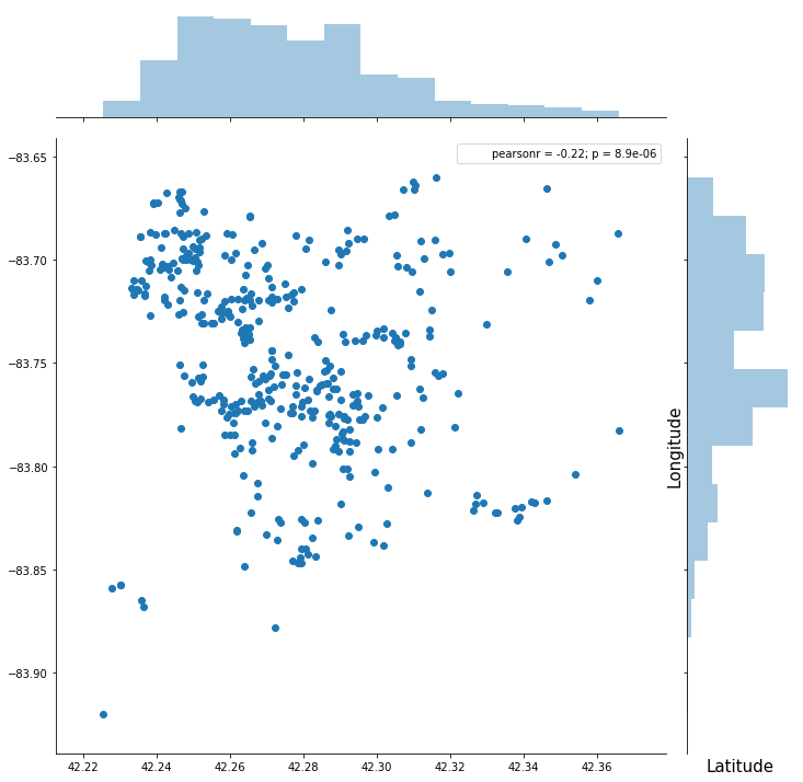
Plotting by each house’s location:

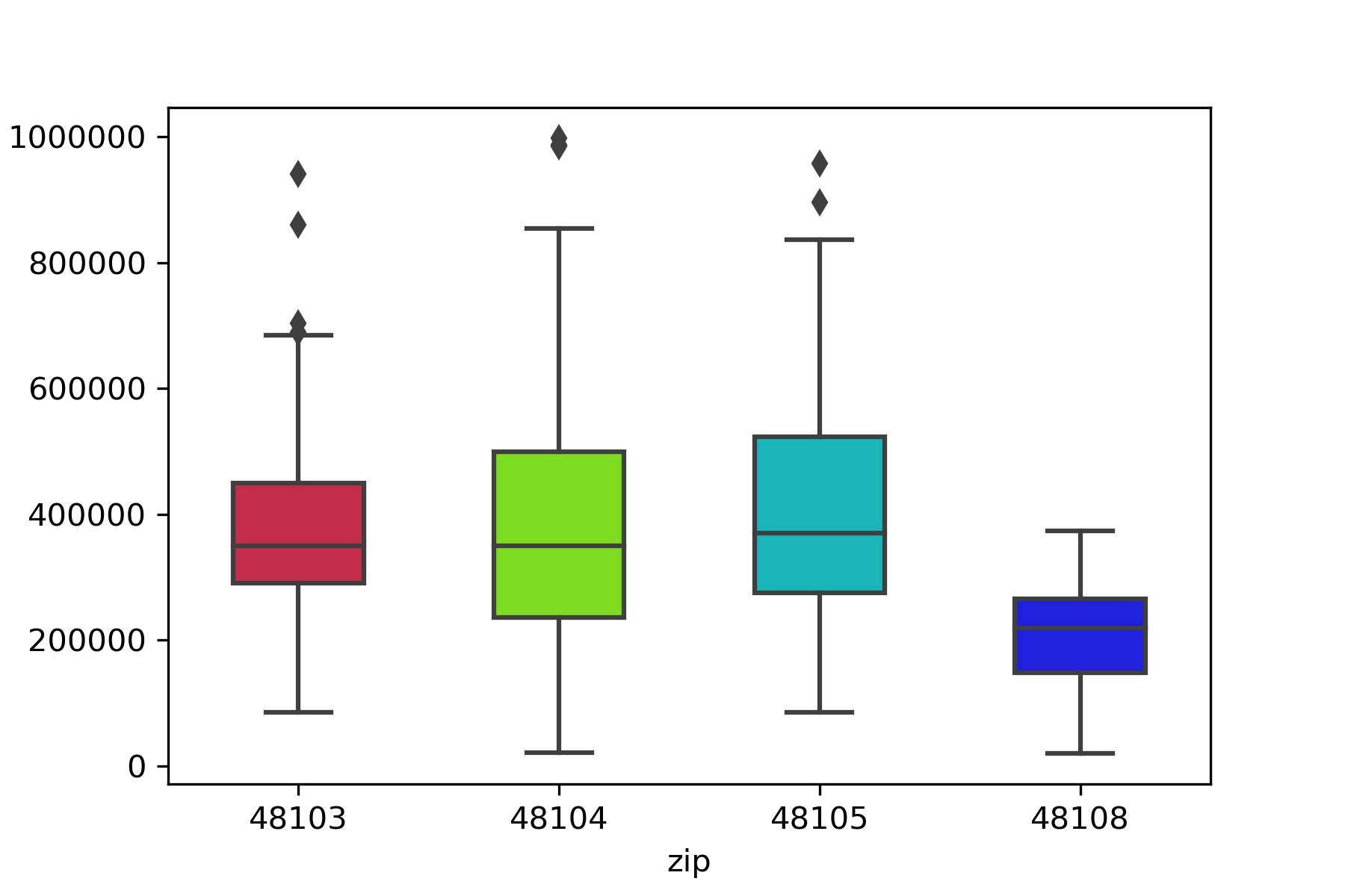
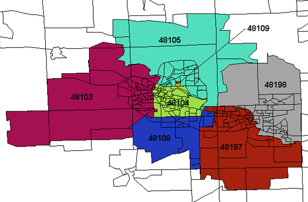
Plotting prices by zipcode:


I didn’t end up using zipcode or geographic location in my model. long and lat were not predictive, and while zipcode was a little bit, it didn’t make sense to me to use such arbitrary boundaries. (If I were doing more than one city it would make more sense to use.)
Feature Engineering
I applied a standard scaler to all of my features, which transforms the variables so that the mean is 0 and the standard distribution is 1.
I explored using polynomial features as well as interactions, but those didn’t seem to improve my model much, so I decided to keep it simple and leave those out.
Model
The model that I choose to use is an ordinary least squares linear regression. To account for collinearity of variables (for example, you might expect number of bathrooms and bedrooms to rise as the overall sq footage rises), I used a method called Ridge Regularization. Ridge Regularization– or L2 regularization– puts a penalty on large coefficients (also known as Betas, β), without making the coefficients zero. L1 regularization tends to “zero-out” some coefficients in favor of others, I didn’t want that.
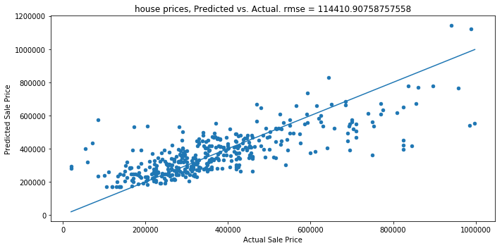
Here’s how my model did:

It had an r-squared value of 0.62, which means that my model accounts for 62% of the variation in home prices in Ann Arbor. I think with more features and more data points I can increase that even more.
Insights
According to my model, all else equal,
| One additional: | correlates with an increase in value of: |
|---|---|
| Bedroom | $3,157 |
| Bathroom | $26,818 |
| House square foot | $49 |
| Lot square foot | $0.30 |
| Year older | $12 |
Most surprising to me was how valuable a bathroom is! $26k seems like a lot. I suspect that this is because more expensive homes tend to have more bathrooms, rather than one bathroom being worth more than $25,000. If I can collect more features, I suspect that that number will go down.
Based on this model, here is the formula for computing a house price in Ann Arbor:
Price in dollars = 379,428 - 12.1x(year) +3,157x(#bedrooms) + 26,818x(#bathrooms) + 0.29x(lot size in sq ft.) + 49 x (house square footage)